Exploratory Data Analysis Guide for Beginners

You load your dataset. Everything looks structured. Rows are filled. Columns have names. At first glance, the data seems ready.

Then problems start to appear.

Some values are missing. Some numbers look unusually high. Some columns do not make sense together. If you move straight into modeling at this point, your results will fail.

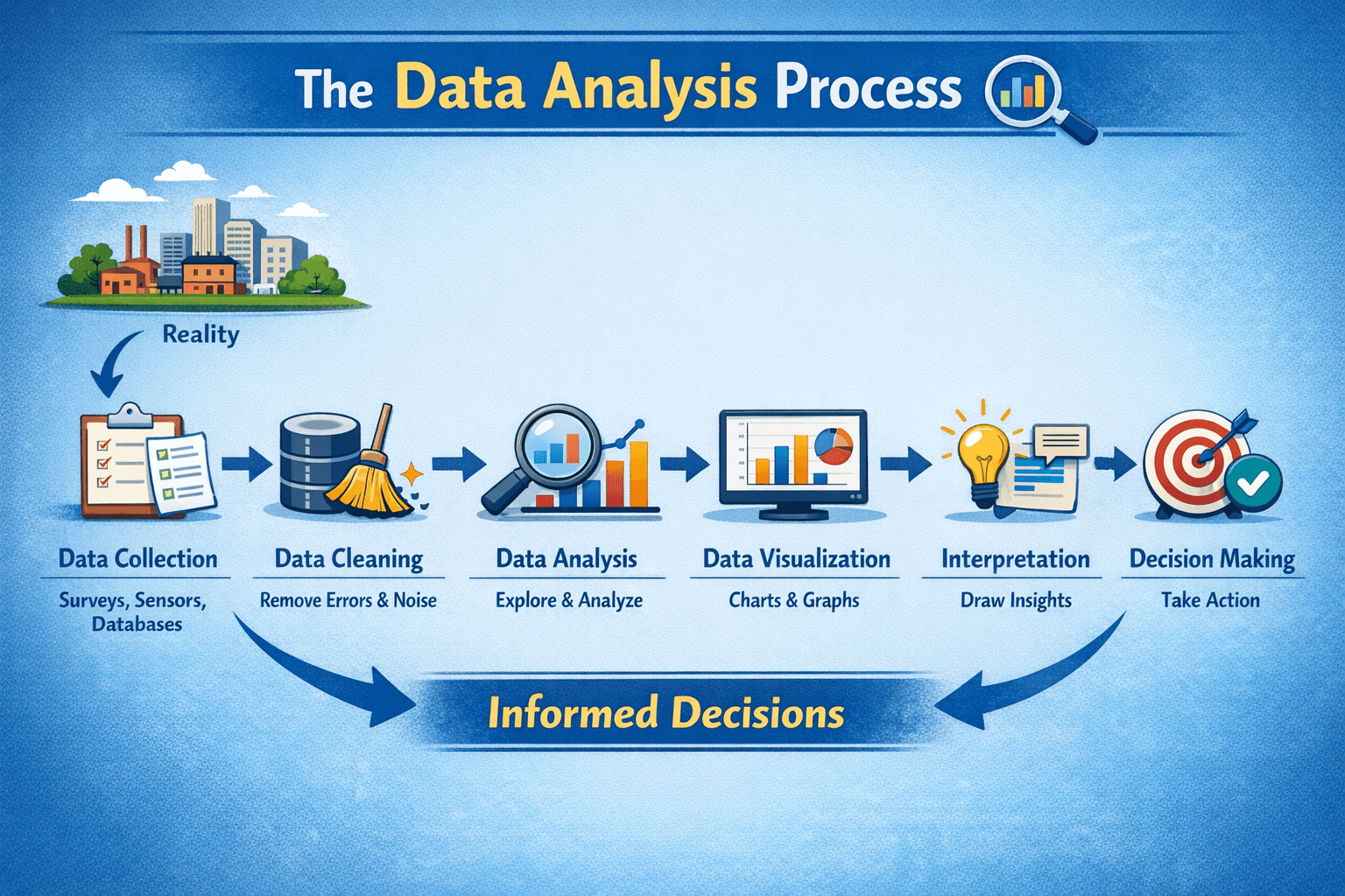
This is why Exploratory Data Analysis exists.

EDA gives you control over your data before you depend on it. You understand what you are working with instead of guessing.

---

What is EDA

Exploratory Data Analysis is the process of studying your dataset to understand its structure, quality, and patterns before building models.

In a real scenario, imagine you are working on an e commerce dataset. You want to predict customer spending.

Without EDA:

• You trust the data blindly
• You train a model
• You get poor predictions

With EDA:

• You notice missing values in income
• You find extreme outliers in purchase amount
• You detect strong relation between age and spending

EDA changes your approach from assumption to evidence.

---

Why visualization matters

Numbers alone rarely tell the full story. Visualization makes patterns visible.

Suppose you are analyzing user ages.

If you look at raw numbers, you see a long list. No clear insight appears. When you plot a histogram, a pattern emerges. Most users fall between 20 and 30. A few values sit far away, which signals possible outliers.

Now consider a business case.

You plot revenue against time. The graph shows a sudden spike in one month. This could indicate a marketing campaign or a data issue. Without visualization, this insight stays hidden.

Visualization helps you:

• detect skewed distributions
• identify clusters
• spot anomalies
• understand relationships

---

Steps involved in EDA

EDA follows a structured flow. Each step builds on the previous one.

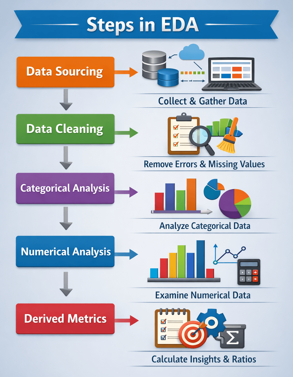
Data sourcing

Data comes from different sources such as APIs, databases, or files.

The source affects reliability. Data from user input often contains errors. Data from systems may contain duplicates or logs.

In a real use case, a company collects customer data from multiple platforms. Some fields overlap. Some conflict. EDA starts by understanding where the data comes from.

Data cleaning

Cleaning is one of the most important steps.

You handle:

• missing values
• duplicate records
• incorrect formats

Example:

A dataset has a column for age. Some entries are empty. If you ignore them, calculations break.

You replace missing values with the median. This keeps the distribution stable.

Another example involves salary stored as text. You convert it into numeric format to make it usable.

Categorical analysis

Categorical variables represent groups.

In a marketing dataset, you might analyze customer regions. If one region dominates the dataset, your model might become biased.

You check frequency distribution. You look for imbalance. This helps you understand how categories affect your analysis.

Numerical analysis

Numerical columns give measurable insights.

You calculate:

• mean to understand average
• median to understand typical value
• standard deviation to measure spread

Example:

In salary data, a high mean but lower median suggests skewness. A few high values pull the average up.

This tells you that most users earn less than the average.

Derived metrics

Raw data often lacks useful context. You create new features to improve it.

In an e commerce dataset:

• Revenue equals price multiplied by quantity
• Customer lifetime value combines multiple transactions

These derived metrics help you see deeper patterns.

---

Handling Missing Values

Missing data is common in real datasets. Ignoring it can lead to biased analysis and poor model performance. There are multiple ways to handle missing values depending on the situation.

1. Delete Rows or Columns

If a row or column has too many missing values, removing it may be simplest.

• Delete rows if only a few entries are missing.
• Delete columns if most values are missing and the column is not critical.

Example:
If 2 out of 1000 rows have missing age, removing them won’t affect results much.

2. Replace with Mean, Median, or Mode

This is a simple imputation method.

• Mean for numeric data without extreme outliers.
• Median for numeric data with skewed distribution.
• Mode for categorical data.

Example:
If income has missing values, replacing them with median income keeps the data realistic.

3. Algorithmic Imputation

Use statistical or machine learning models to estimate missing values.

• Linear regression or k-nearest neighbors can predict missing numeric values.
• Classification models can predict missing categories.

Example:
Predict missing age using other features like occupation, income, or location.

4. Predicting the Missing Values

For complex datasets, you can train a model specifically to predict missing entries based on available data.

• Treat missing value prediction as a mini supervised learning task.
• Ensures imputed values preserve relationships in the dataset.

Example:
In a customer dataset, predict missing credit scores using age, income, and transaction history.

This approach keeps the data complete and usable while reducing bias. Choosing the right method depends on how many values are missing and the type of feature.

---

Feature scaling and standardization

Features often exist on different scales.

In a housing dataset:

• Area ranges in thousands
• Number of rooms ranges in single digits

If you use these directly, models focus more on larger values.

Feature scaling solves this problem.

Standardization

Standardization transforms data to have a mean of zero and standard deviation of one.

z = (x - mean) / standard deviation

Use case:

In a dataset with mixed features, standardization ensures each feature contributes equally. This is useful in algorithms like logistic regression and clustering.

Normalization

Normalization scales data between zero and one.

x' = (x - min) / (max - min)

Use case:

In image processing or neural networks, normalized inputs help models converge faster.

---

Outliers and their treatment

Outliers are values that differ significantly from others.

In a financial dataset, most transactions fall under a certain range. A few transactions are extremely high. These could be fraud or data errors.

Outliers affect:

• mean values
• model accuracy
• data distribution

You detect outliers using:

• box plots
• z score
• distribution plots

You treat them based on context:

• remove them if they are errors
• cap them if they are extreme but valid
• transform data to reduce impact

---

Handling invalid values

Invalid values break your analysis pipeline.

Examples include:

• negative age
• text in numeric columns
• impossible values

In a real dataset, you might find age recorded as negative due to entry errors. You either remove such rows or replace them using logical rules.

Handling invalid values ensures consistency.

---

Types of data

Understanding data types helps you apply the correct methods.

Qualitative data represents categories.

Nominal data has no order. For example, colors or gender.
Ordinal data has order. For example, ratings like low, medium, high.

Quantitative data represents numbers.

Discrete data counts items, such as number of purchases.
Continuous data measures values, such as height or temperature.

Each type requires a different analysis approach.

---

Types of analysis

EDA includes multiple levels of analysis.

Univariate analysis focuses on a single variable. You study distribution and spread.

Bivariate analysis examines relationships between two variables. For example, age and income.

Multivariate analysis studies multiple variables together. This helps identify combined effects.

In a business use case, multivariate analysis helps understand how age, income, and location together influence purchasing behavior.

---

Feature binning

Continuous values are sometimes too detailed.

Feature binning groups them into ranges.

In a banking dataset, age can be grouped into categories. This simplifies analysis and improves model performance in some cases.

Binning also helps reduce noise.

---

Feature encoding

Machine learning models work with numbers, not categories.

Encoding converts categorical data into numeric form.

In a dataset with product categories, each category is assigned a number or converted into multiple binary columns.

This step is necessary before training models.

---

Use cases of EDA

EDA applies across domains.

In business analytics, it reveals sales patterns and seasonal trends.
In finance, it helps detect unusual transactions and fraud.
In e commerce, it analyzes customer behavior and purchase patterns.
In healthcare, it studies patient records and risk factors.

In machine learning, EDA prepares clean and reliable input, which directly affects model performance.

---

Final thoughts

EDA is the foundation of data analysis.

You do not rush into building models. You first understand your data. You question it. You clean it. You reshape it.

Strong analysis starts with strong understanding.

---